── Attaching core tidyverse packages ──────────────────────── tidyverse 2.0.0 ──
✔ dplyr     1.1.4     ✔ readr     2.1.5
✔ forcats   1.0.0     ✔ stringr   1.5.1
✔ ggplot2   3.5.2     ✔ tibble    3.2.1
✔ lubridate 1.9.4     ✔ tidyr     1.3.1
✔ purrr     1.0.4
── Conflicts ────────────────────────────────────────── tidyverse_conflicts() ──
✖ dplyr::filter() masks stats::filter()
✖ dplyr::lag()    masks stats::lag()
ℹ Use the conflicted package (<http://conflicted.r-lib.org/>) to force all conflicts to become errors
Code
library(MplusAutomation)
Version:  1.1.1
We work hard to write this free software. Please help us get credit by citing:

Hallquist, M. N. & Wiley, J. F. (2018). MplusAutomation: An R Package for Facilitating Large-Scale Latent Variable Analyses in Mplus. Structural Equation Modeling, 25, 621-638. doi: 10.1080/10705511.2017.1402334.

-- see citation("MplusAutomation").
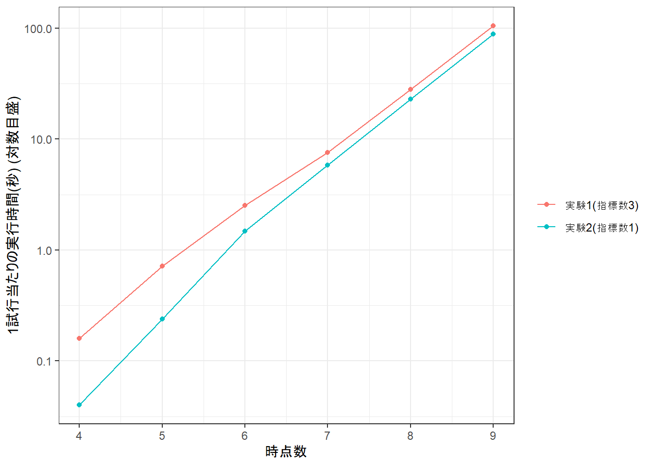
g <-ggplot(data = dfTime, aes(x = nNumTime, y = gSecond, group = fExperiment, color = fExperiment))g <- g +geom_point()g <- g +geom_line()g <- g +labs(x ="時点数", y ="1試行当たりの実行時間(秒) (対数目盛)", color =NULL)g <- g +scale_y_log10()g <- g +scale_x_continuous(breaks = anT)g <- g +theme_bw()print(g)
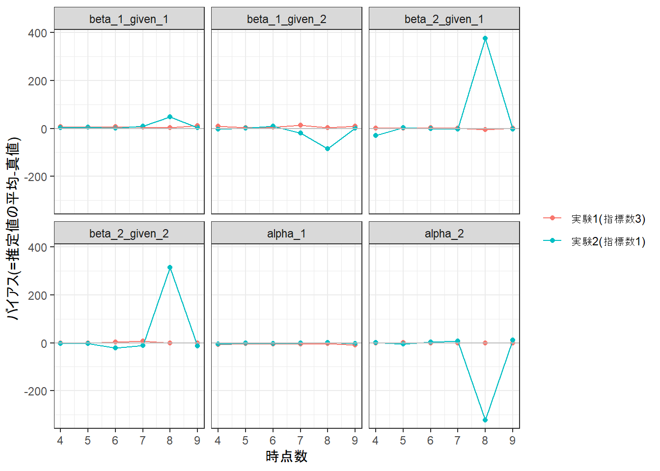
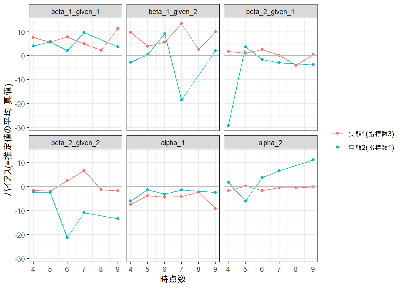
g <-ggplot(data = dfPlot |> dplyr::filter(!(nExperiment ==2& nNumTime ==8)),aes(x = nNumTime, y = gBias, group = fExperiment, color = fExperiment))g <- g +geom_point()g <- g +geom_line()g <- g +geom_hline(yintercept =0, color ="gray")g <- g +labs(x ="時点数", y ="バイアス(=推定値の平均-真値)", color =NULL)g <- g +facet_wrap(~ fParam)g <- g +theme_bw()print(g)
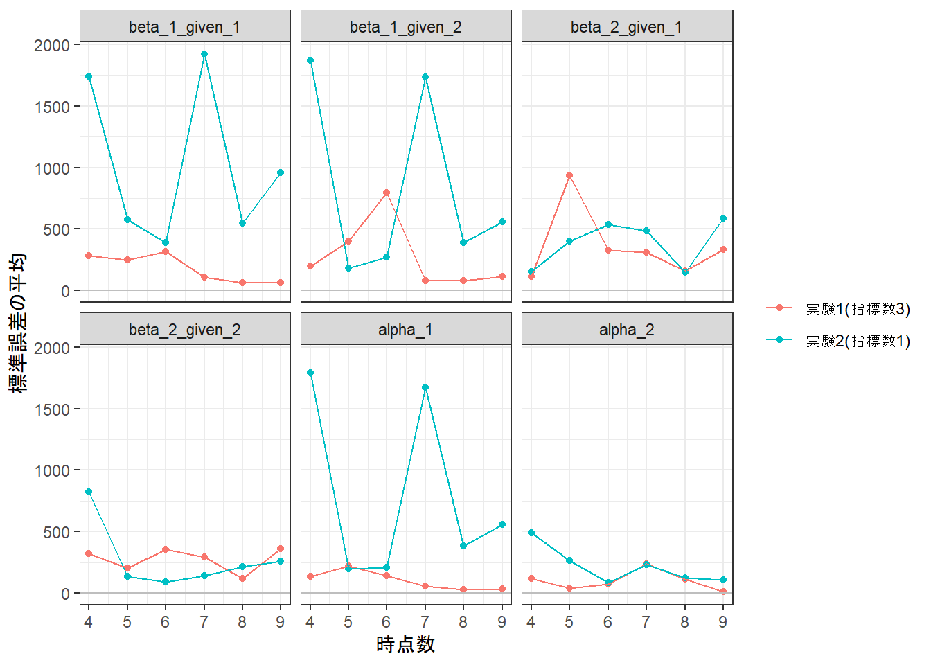
g <-ggplot(data = dfPlot, aes(x = nNumTime, y = average_se, group = fExperiment, color = fExperiment))g <- g +geom_point()g <- g +geom_line()g <- g +geom_hline(yintercept =0, color ="gray")g <- g +labs(x ="時点数", y ="標準誤差の平均", color =NULL)g <- g +facet_wrap(~ fParam)g <- g +theme_bw()print(g)
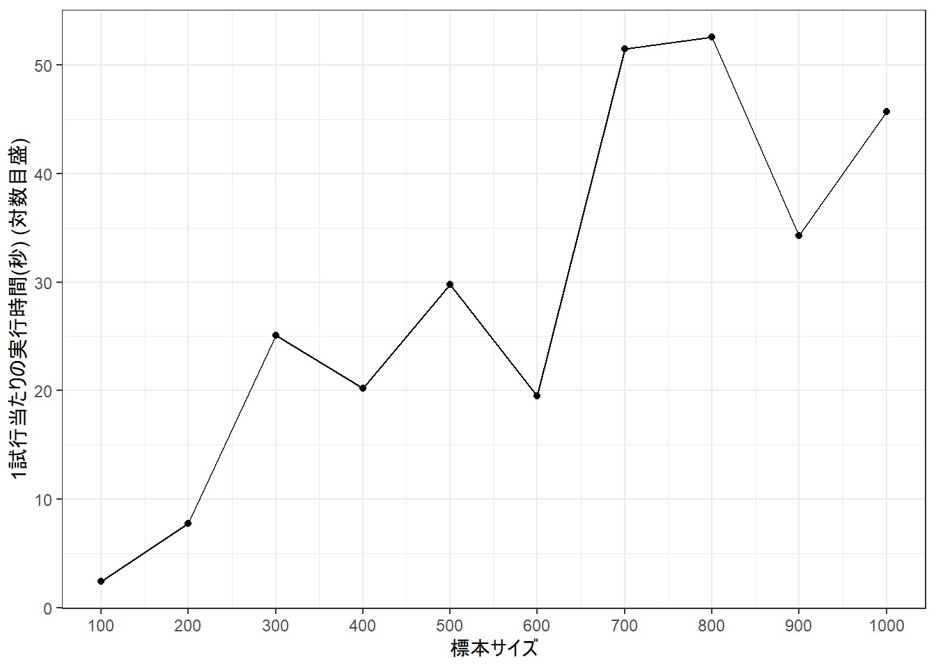
g <-ggplot(data = dfTime_3, aes(x = nN, y = gSecond))g <- g +geom_point()g <- g +geom_line()g <- g +labs(x ="標本サイズ", y ="1試行当たりの実行時間(秒) (対数目盛)", color =NULL)# g <- g + scale_y_log10()g <- g +scale_x_continuous(breaks =seq(100, 1000, 100))g <- g +theme_bw()print(g)
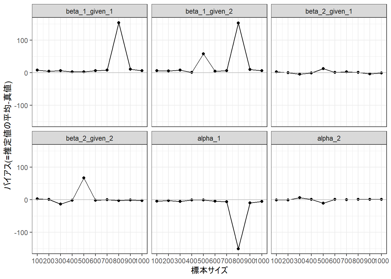
lParam <-lapply( lResult_3, function(lIn){ lIn$parameters$unstandardized |> dplyr::select(-mse) # なぜかしらんが型が異なる }) dfParam <-bind_rows(lParam, .id ="sOutput") |>separate(sOutput, c("sDummy1", "nExperiment", "nN", "sDummy2"), sep ="[_\\.]") |>mutate(nN =as.integer(nN) ) |> dplyr::select(nN, paramHeader, param, average, average_se)# print(dfParam)# stop()dfTemplate <-tibble(paramHeader =c("C2#1.ON", "C2#1.ON", "C2#2.ON", "C2#2.ON", "Means", "Means"),param =c("C1#1", "C1#2", "C1#1", "C1#2", "C2#1", "C2#2"),sParam =c("beta_1_given_1", "beta_1_given_2", "beta_2_given_1", "beta_2_given_2", "alpha_1", "alpha_2"),gTrue =c(1.61, 2.19, 0.69, 2.89, -1.10, -1.10)) |>mutate(fParam =factor(sParam, levels = sParam))dfPlot <- dfParam |>inner_join(dfTemplate, by =c("paramHeader", "param")) |>mutate(gBias = average - gTrue) # print(dfPlot)g <-ggplot(data = dfPlot, aes(x = nN, y = gBias))g <- g +geom_point()g <- g +geom_line()g <- g +geom_hline(yintercept =0, color ="gray")g <- g +scale_x_continuous(breaks =seq(100, 1000, 100))g <- g +labs(x ="標本サイズ", y ="バイアス(=推定値の平均-真値)", color =NULL)g <- g +facet_wrap(~ fParam)g <- g +theme_bw()print(g)
うわあ… n=500, 800で滅茶苦茶な推定値になっている… (ドン引き)
この2点を抜いて描きなおしてみても、
Code
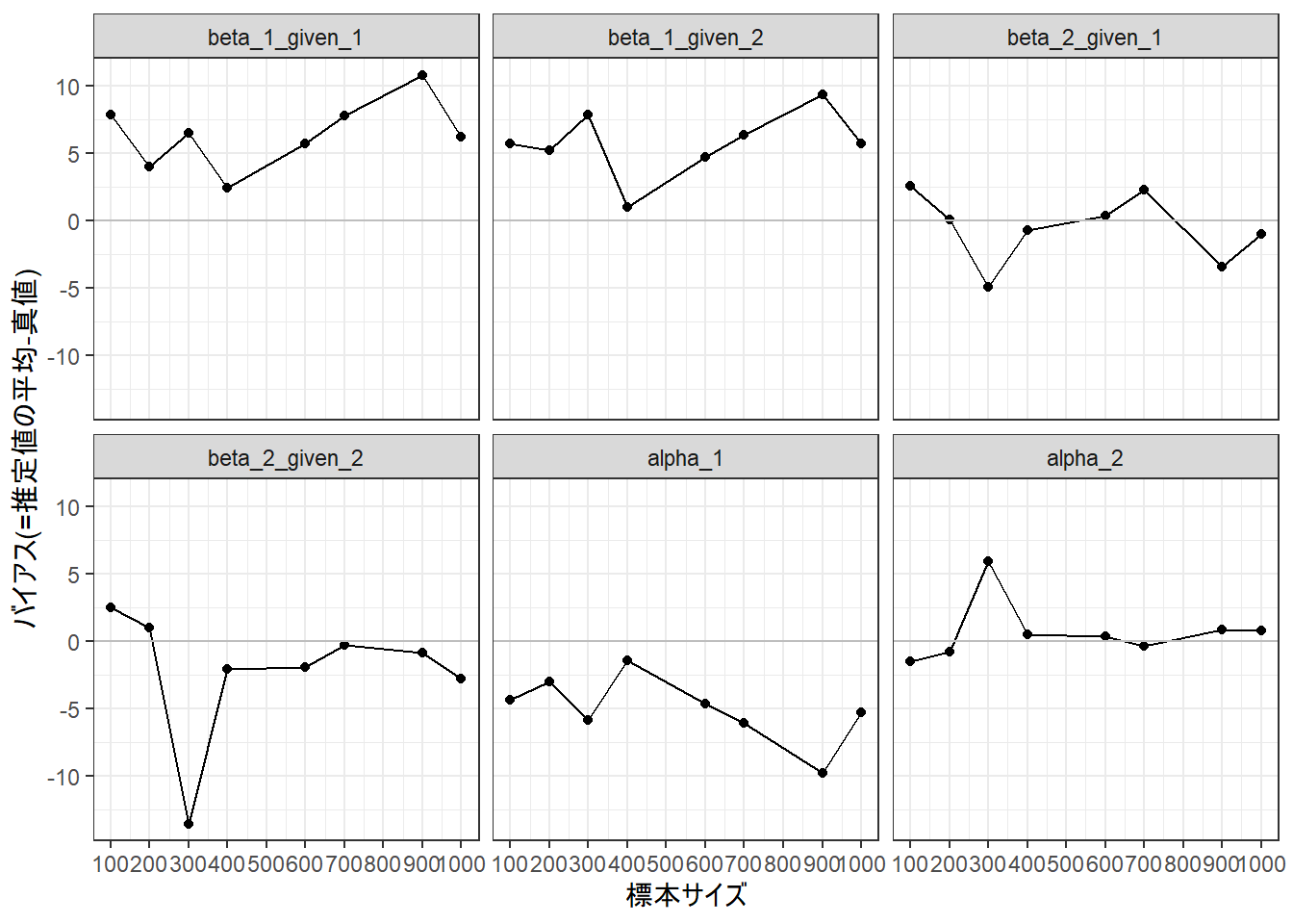
g <-ggplot(data = dfPlot |> dplyr::filter(!(nN %in%c(500, 800))),aes(x = nN, y = gBias))g <- g +geom_point()g <- g +geom_line()g <- g +geom_hline(yintercept =0, color ="gray")g <- g +scale_x_continuous(breaks =seq(100, 1000, 100))g <- g +labs(x ="標本サイズ", y ="バイアス(=推定値の平均-真値)", color =NULL)g <- g +facet_wrap(~ fParam)g <- g +theme_bw()print(g)
バイアスは結構大きく、標本サイズとのあいだでの明確な関係はみられない。ええええ!?
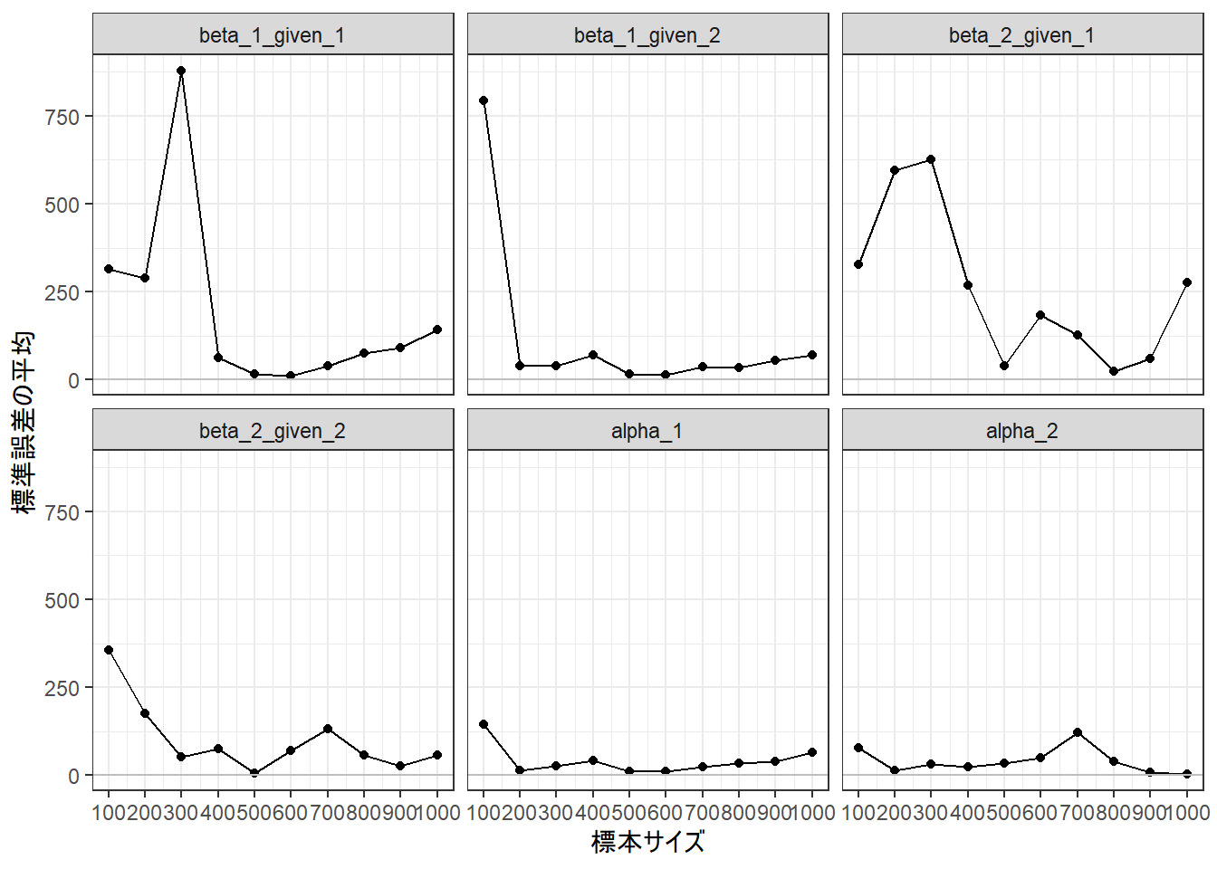
8.3 推定のばらつき
標準誤差はどうか。
Code
g <-ggplot(data = dfPlot, aes(x = nN, y = average_se))g <- g +geom_point()g <- g +geom_line()g <- g +geom_hline(yintercept =0, color ="gray")g <- g +scale_x_continuous(breaks =seq(100, 1000, 100))g <- g +labs(x ="標本サイズ", y ="標準誤差の平均", color =NULL)g <- g +facet_wrap(~ fParam)g <- g +theme_bw()print(g)